-matrix2stata-
Description
The command -matrix2stata- converts roweq, rownames and content from a matrix into variables. This makes it eg possible to do graphs of the content of one or more matrices. The difference from -svmat- is that it adds roweq and rownames as variables for grouping.
The matrices might have been generated from -sumat-.
Installation
To install use the command: ssc install matrixtools
Demonstration
The dataset
The dataset in this example is auto with a value label:
sysuse auto, clear
label define rep78 1 "1 repair" 2 "2 repairs" 3 "3 repairs" 4 "4 repairs" 5 "5 repairs"
label values rep78 rep78
The command -sumat- is used to generate a matrix with some content to plot:
sumat price  if foreign == "Foreign":origin, statistics(mean ci) rowby(rep78) roweq(Foreign) full
matrix out = r(sumat)
sumat price  if foreign == "Domestic":origin, statistics(mean ci) rowby(rep78) roweq(Domestic) full
matrix out = out \ r(sumat)
And the matrix looks like
matprint out
--------------------------------------------------------------------
                                            mean  ci95% lb  ci95% ub
--------------------------------------------------------------------
Foreign   Repair record 1978(1 repair)
          Repair record 1978(2 repairs)
          Repair record 1978(3 repairs)  4828.67   3373.89   6283.45
          Repair record 1978(4 repairs)  6261.44   5022.69   7500.20
          Repair record 1978(5 repairs)  6292.67   4485.82   8099.51
Domestic  Repair record 1978(1 repair)   4564.50   3840.29   5288.71
          Repair record 1978(2 repairs)  5967.63   3487.30   8447.95
          Repair record 1978(3 repairs)  6607.07   5226.06   7988.09
          Repair record 1978(4 repairs)  5881.56   4841.46   6921.66
          Repair record 1978(5 repairs)  4204.50   3772.33   4636.67
--------------------------------------------------------------------
Now -matrix2stata- is used to move the content of the matrix out to the dataset. The option clear clears the dataset before inserting the matrix.
matrix2stata out, clear
The command -matrix2stata- returns the following stored results:
display "`:r(macros)'"
variable_names
display "`r(variable_names)'"
out_eq out_names out_mean out_ci95__lb out_ci95__ub
The current dataset now looks like:
list
     +------------------------------------------------------------------------------+
     |   out_eq                       out_names    out_mean   out_ci~lb   out_ci~ub |
     |------------------------------------------------------------------------------|
  1. |  Foreign    Repair record 1978(1 repair)           .           .           . |
  2. |  Foreign   Repair record 1978(2 repairs)           .           .           . |
  3. |  Foreign   Repair record 1978(3 repairs)   4828.6667   3373.8855   6283.4478 |
  4. |  Foreign   Repair record 1978(4 repairs)   6261.4444   5022.6874   7500.2015 |
  5. |  Foreign   Repair record 1978(5 repairs)   6292.6667   4485.8221   8099.5113 |
     |------------------------------------------------------------------------------|
  6. | Domestic    Repair record 1978(1 repair)      4564.5   3840.2933   5288.7067 |
  7. | Domestic   Repair record 1978(2 repairs)    5967.625   3487.3029   8447.9471 |
  8. | Domestic   Repair record 1978(3 repairs)   6607.0741   5226.0617   7988.0865 |
  9. | Domestic   Repair record 1978(4 repairs)   5881.5556   4841.4554   6921.6557 |
 10. | Domestic   Repair record 1978(5 repairs)      4204.5   3772.3279   4636.6721 |
     +------------------------------------------------------------------------------+
The variable name Price appears unnecessary in the variable out_names. This is remedied by the utility commands -strofnum- and -strtonum-:
strofnum out_names
replace out_names = subinstr(out_names, ", Price", "",.)
strtonum out_names
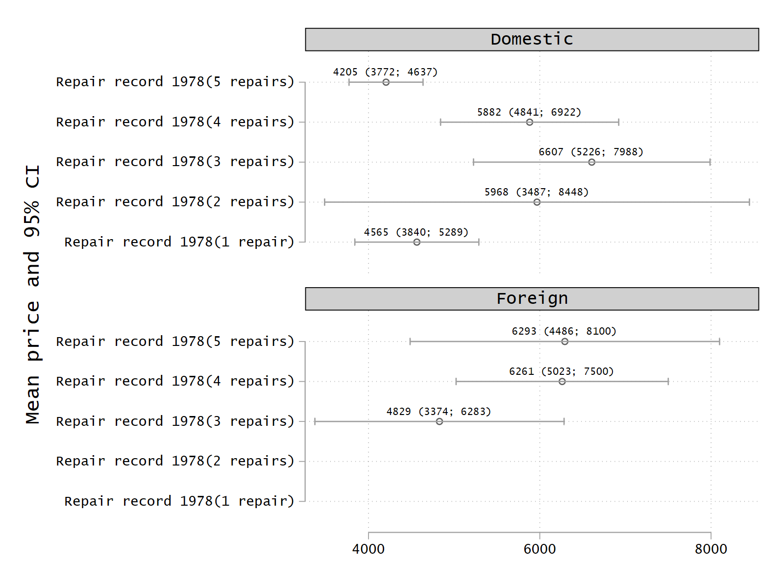
To create a CI plot
To add estimate and CI as labels a marker label variable is made and some labelling is done:
generate lbl = string(out_mean, "%6.0f") + " (" + string(out_ci95__lb, "%6.0f") + "; " + string( out_ci95__ub, "%6.0f") + ")"
label variable out_eq "Origin"
label variable out_names "Repair record 1978"
Now the graph can be generated:
twoway  (scatter out_names out_mean, mlabel(lbl) mlabsize(vsmall) mlabposition(12)) ///
                (rcap out_ci95__lb out_ci95__ub out_names, horizontal) ///
                , yscale(range(.5 5.5)) ///
                ylabel(1(1)5, angle(zero) valuelabel) ///
                by(out_eq, legend(off) cols(1) note("")) ytitle(Mean price and 95% CI) name(g1, replace)
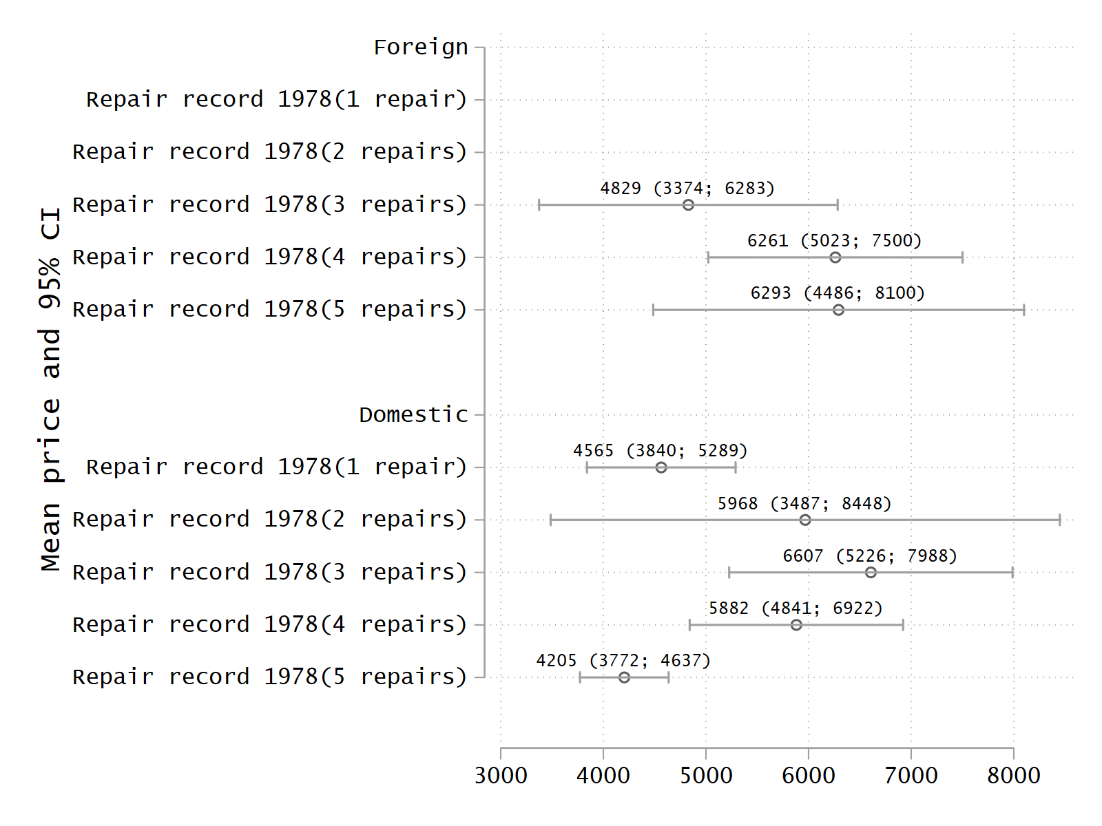
To create a slightly different CI plot
An alternative using the option ziprows is:
sysuse auto, clear
label define rep78 1 "1 repair" 2 "2 repairs" 3 "3 repairs" 4 "4 repairs" 5 "5 repairs"
label values rep78 rep78
sumat price  if foreign == "Foreign":origin, statistics(mean ci) rowby(rep78) roweq(Foreign) full
matrix out = r(sumat)
sumat price  if foreign == "Domestic":origin, statistics(mean ci) rowby(rep78) roweq(Domestic) full
matrix out = out \ r(sumat)
matrix2stata out, clear ziprows
Now the dataset looks like:
list
     +------------------------------------------------+
     | out_rowe~s    out_mean   out_ci~lb   out_ci~ub |
     |------------------------------------------------|
  1. |    Foreign           .           .           . |
  2. | Repair rec           .           .           . |
  3. | Repair rec           .           .           . |
  4. | Repair rec   4828.6667   3373.8855   6283.4478 |
  5. | Repair rec   6261.4444   5022.6874   7500.2015 |
     |------------------------------------------------|
  6. | Repair rec   6292.6667   4485.8221   8099.5113 |
  7. |          7           .           .           . |
  8. |   Domestic           .           .           . |
  9. | Repair rec      4564.5   3840.2933   5288.7067 |
 10. | Repair rec    5967.625   3487.3029   8447.9471 |
     |------------------------------------------------|
 11. | Repair rec   6607.0741   5226.0617   7988.0865 |
 12. | Repair rec   5881.5556   4841.4554   6921.6557 |
 13. | Repair rec      4204.5   3772.3279   4636.6721 |
 14. |          0           .           .           . |
     +------------------------------------------------+
And the graph is generated by:
generate lbl = string(out_mean, "%6.0f") + " (" + string(out_ci95__lb, "%6.0f") + "; " + string( out_ci95__ub, "%6.0f") + ")"
twoway      (scatter out_roweqnames out_mean, mlabel(lbl) mlabsize(vsmall) mlabposition(12)) ///
                (rcap out_ci95__lb out_ci95__ub out_roweqnames, horizontal) ///
                , ylabel(1(1)6 8(1)13, angle(zero) valuelabel) ///
                legend(off) ytitle(Mean price and 95% CI) name(g2, replace)
Last update: 2022-04-19, Stata version 17