Prediction modelling in logistic regression
Objective
To demonstrate how to build a prediction model in logistic regression using tools available in Stata 12 and above.
The data
The ICU data set consists of a sample of 200 subjects who were part of a much larger study on survival of patients following admission to an adult intensive care.
The major goal of this study was to develop a logistic regression model to predict the probability of survival to hospital discharge of these patients and to study the risk factors associated with ICU mortality based on the risk factors in this dataset.
The ICU dataset used in this document
use icu, clear
The dataset can be summarised as:
metadata *
| Name | Index | Label | Value Label Name | Format | Value Label Values | n | unique | missing |
|---|---|---|---|---|---|---|---|---|
| sta | 1 | Vital Status | sta | %27.0g | 0 "Alive at hospital discharge" 1 "Dead at hospital discharge" | 200 | 2 | 0 |
| age | 2 | Age in years | %9.0g | 200 | 64 | 0 | ||
| sex | 3 | Sex | sex | %9.0g | 0 "female" 1 "male" | 200 | 2 | 0 |
| race | 4 | Race | race | %9.0g | 1 "white" 2 "black" 3 "other" | 200 | 3 | 0 |
| can | 5 | Cancer part of present problem | can | %9.0g | 0 "no" 1 "yes" | 200 | 2 | 0 |
| crn | 6 | History of chronic renal failure | crn | %9.0g | 0 "no" 1 "yes" | 200 | 2 | 0 |
| cpr | 7 | CPR prior to ICU admission | cpr | %9.0g | 0 "no" 1 "yes" | 200 | 2 | 0 |
| sys | 8 | Systolic blood pressure mm Hg | %9.0g | 200 | 63 | 0 | ||
| hra | 9 | Heart rate at ICU admission beats/min | %9.0g | 200 | 81 | 0 | ||
| typ | 10 | Type of admission | typ | %9.0g | 0 "elective" 1 "emergency" | 200 | 2 | 0 |
| po2 | 11 | PO2 from initial blood gases | po2 | %9.0g | 0 ">60" 1 "=<60" | 200 | 2 | 0 |
| ph | 12 | PH from initial blood gases | ph | %9.0g | 0 ">7.25" 1 "=<7.25" | 200 | 2 | 0 |
| pco | 13 | PCO2 from initial blood gases | pco | %9.0g | 0 "<=45" 1 ">45" | 200 | 2 | 0 |
| locd | 14 | Level of consciousness at ICU admission* | locd | %22.0g | 0 "no coma or deep stupor" 1 "coma or deep stupor" | 200 | 2 | 0 |
Screening for risk factors to use
In prediction modeling the objective is to obtain the most parsimonious and yet the best fitting model possible.
Here the outcome is dichotome Alive/Dead at hospital discharge.
Based on significant main effects a base of risk factors are chosen at first.
Significance can be decided using eg t-test or similar when the risk factor is continuous and twosided chisquare tests when the risk factor is categorical or by fitting simple logistic/logistic regression.
The first can be done eg using the command -basetable- and the second by running through the a set of simple logistic regressions.
If necessary risk factors due to clinical reasons can also be chosen. However, they will usually have no effect in the predictions if the aren't significant in the final prediction model.
Using basetable
The -command- can do comparisons between the outcome (Alive/Dead at hospital discharge) and the risk factors.
When the risk factor is categorical chisquare is used and since the median is reported a Kruskal-Wallis test is used.
basetable sta age(%6.1f) sex(male) race(c) can(yes) crn(yes) cpr(yes) sys(%6.1f) ///
        hra(%6.1f) typ(emergency) po2(=<60) ph(=<7.25) pco(<=45) ///
        locd(coma or deep stupor), continuousreport(iqi)
| Columns by: Vital Status | Alive at hospital discharge | Dead at hospital discharge | Total | P-value |
|---|---|---|---|---|
| n (%) | 160 (80.0) | 40 (20.0) | 200 (100.0) | |
| Age in years, median (iqi) | 61.0 (41.3; 71.0) | 68.0 (55.5; 75.0) | 63.0 (46.2; 72.0) | 0.01 |
| Sex (male), n (%) | 60 (37.5) | 16 (40.0) | 76 (38.0) | 0.77 |
| Race, n (%) | ||||
| white | 138 (86.3) | 37 (92.5) | 175 (87.5) | |
| black | 14 (8.8) | 1 (2.5) | 15 (7.5) | |
| other | 8 (5.0) | 2 (5.0) | 10 (5.0) | 0.40 |
| Cancer part of present problem (yes), n (%) | 16 (10.0) | 4 (10.0) | 20 (10.0) | 1.00 |
| History of chronic renal failure (yes), n (%) | 11 (6.9) | 8 (20.0) | 19 (9.5) | 0.01 |
| CPR prior to ICU admission (yes), n (%) | 6 (3.8) | 7 (17.5) | 13 (6.5) | 0.00 |
| Systolic blood pressure mm Hg, median (iqi) | 132.0 (112.0; 154.0) | 126.0 (87.0; 140.0) | 130.0 (110.0; 150.0) | 0.01 |
| Heart rate at ICU admission beats/min, median (iqi) | 95.0 (80.0; 117.5) | 96.0 (81.0; 121.3) | 96.0 (80.0; 118.7) | 0.63 |
| Type of admission (emergency), n (%) | 109 (68.1) | 38 (95.0) | 147 (73.5) | 0.00 |
| PO2 from initial blood gases (=<60), n (%) | 11 (6.9) | 5 (12.5) | 16 (8.0) | 0.24 |
| PH from initial blood gases (=<7.25), n (%) | 9 (5.6) | 4 (10.0) | 13 (6.5) | 0.32 |
| PCO2 from initial blood gases (<=45), n (%) | 144 (90.0) | 36 (90.0) | 180 (90.0) | 1.00 |
| Level of consciousness at ICU admission* (coma or deep stupor), n (%) | 2 (1.3) | 13 (32.5) | 15 (7.5) | 0.00 |
Significant risk factors are here age, cpr, sys, typ and locd.
Estimating crude main effects
Repeatedly using logistic or logistic eg by
foreach var of varlist age-locd {
        logistic sta `var', or
}
logistic sta, or
The last logistic outside the foreach loop generates the crude estimate.
Summary below is inspired by powerpoint presentation of S. Lemeshow in 2015.
| Estimate | lb | ub | p | Loglikelihood | G | f | P | |
|---|---|---|---|---|---|---|---|---|
| age | 1.028 | 1.007 | 1.049 | 0.009 | -96.153 | 7.855 | 1 | 0.005 |
| sex | 1.111 | 0.547 | 2.258 | 0.771 | -100.038 | 0.084 | 1 | 0.771 |
| race(1) | 1.000 | -98.951 | 2.260 | 2 | 0.323 | |||
| race(2) | 0.266 | 0.034 | 2.092 | 0.208 | -98.951 | 2.260 | 2 | 0.323 |
| race(3) | 0.932 | 0.190 | 4.579 | 0.931 | -98.951 | 2.260 | 2 | 0.323 |
| can | 1.000 | 0.315 | 3.174 | 1.000 | -100.080 | 0.000 | 1 | 1.000 |
| crn | 3.386 | 1.261 | 9.091 | 0.015 | -97.368 | 5.424 | 1 | 0.020 |
| cpr | 5.444 | 1.718 | 17.253 | 0.004 | -96.114 | 7.932 | 1 | 0.005 |
| sys | 0.983 | 0.972 | 0.995 | 0.005 | -95.668 | 8.826 | 1 | 0.003 |
| hra | 1.003 | 0.990 | 1.016 | 0.653 | -99.980 | 0.201 | 1 | 0.654 |
| typ | 8.890 | 2.064 | 38.290 | 0.003 | -92.524 | 15.112 | 1 | 0.000 |
| po2 | 1.935 | 0.632 | 5.927 | 0.248 | -99.460 | 1.240 | 1 | 0.265 |
| ph | 1.864 | 0.543 | 6.395 | 0.322 | -99.626 | 0.910 | 1 | 0.340 |
| pco | 1.000 | 0.315 | 3.174 | 1.000 | -100.080 | 0.000 | 1 | 1.000 |
| locd | 38.037 | 8.125 | 178.074 | 0.000 | -82.778 | 34.604 | 1 | 0.000 |
| sta | 0.250 | 0.177 | 0.354 | -100.080 |
The same risk factors as before (age, cpr, sys, typ and locd) are significant.
Conclusion
age, crn, cpr, sys, typ and locd are included due to statistical significance. can and pco are indcluded due to clinical significance.
Fitting the multivariable model
Fitting the main effects
Based on the fitting of univariate models and clinical considerations we identified as potential variables for a multivariate model.
The results of fitting a model containing these variables follow:
logistic sta age i.crn i.cpr sys i.typ i.locd i.can i.pco, or
estimates store first
estout first, cells("b(fmt(2)) ci(fmt(2)) p(fmt(2))") varwidth(30) eform drop(0* _cons)
| first | |||||
|---|---|---|---|---|---|
| b | lower 95%ci | upper 95%ci | p | ||
| sta | age | 1.04 | 1.01 | 1.07 | 0.00 |
| 1.crn | 1.72 | 0.45 | 6.56 | 0.42 | |
| 1.cpr | 2.21 | 0.41 | 11.95 | 0.36 | |
| sys | 0.98 | 0.97 | 1.00 | 0.04 | |
| 1.typ | 18.50 | 2.92 | 117.25 | 0.00 | |
| 1.locd | 58.21 | 7.92 | 428.10 | 0.00 | |
| 1.can | 9.75 | 1.77 | 53.80 | 0.01 | |
| 1.pco | 0.23 | 0.04 | 1.38 | 0.11 |
We try fitting a new model dropping crn and cpr since they are highly nonsignificant.
logistic sta age sys i.typ i.locd i.can i.pco, or
estimates store second
A likelihood ratio test comparing the first and second is performed:
lrtest first second
Likelihood-ratio test
Assumption: second nested within first

 LR chi2(2) =   1.57
Prob > chi2 = 0.4560
The p-value from the likelihood ratio test is 0.46.
So there is no significant difference between the two models. And hence we choose the smaller. Due to clinical significance are the variables can and locd kept in the model.
Below are the likelihood ratio tests for adding one at a step of the remaining variables.
The code used is:
capture matrix drop tbl
capture matrix drop row
quietly logistic sta age sys typ locd can pco, or
estimates store A
foreach var in sex i.race hra po2 ph {
        quietly logistic sta `var' age sys typ locd can pco, or
        estimates store B
        lrtest B A
        matrix row = r(chi2), r(df), r(p)
        matrix rownames row = `=subinstr("`var'", "i.", "", .)'
        matrix tbl = nullmat(tbl) \ row
}
matrix colnames tbl = "LR chi2" df P
And the results are:
| LR chi2 | df | P | |
|---|---|---|---|
| sex | 1.17 | 1 | 0.28 |
| race | 0.97 | 2 | 0.62 |
| hra | 0.06 | 1 | 0.81 |
| po2 | 0.15 | 1 | 0.70 |
| ph | 4.44 | 1 | 0.04 |
The variable ph is significant and is hence added to the model.
Assessing the scale of the continuous risk factors
Next the continuous risk factors age and sys are examined for non linearity.
There are several methods for doing
-
Quick and Dirty Methods
- Quartile design variables
- Testing for quadratic effect
-
More computer intensive methods
- Smoothed Scatter Plot using -lowess-
- Fractional polynomials using -fp-
- Restricted cubic splines, -mkspline-
The continuous risk factor age
Quartile design for age
The idea is to generate quartiles for the continuous risk factor and look at the development for odds ratios in the 4 groups.
The x-values are eg mean or median of age for each group.
In logistic regression the log odds are linear as a function of the risk factor (age). So the points (mean age, log odds) should appear on a line.
The recipe is:
- Generate group variable by -xtile-
xtile age_grp = age, n(4)
- Calculate and save log odds
quietly logistic sta i.age_grp sys i.typ i.locd i.can i.pco i.ph
matrix logodds = r(table)'
matrix logodds = logodds[1..4, "b"]
- Calculate and save the median (or mean) age
sumat age, stat(p50) rowby(age_grp)
matrix median_age = r(sumat)
matrix tbl = median_age, logodds
- Convert median age and log odds to variables to plot
svmat tbl, names(col)
twoway (connected b p50, sort) (lfit b p50), name(age_quartile_design, replace)
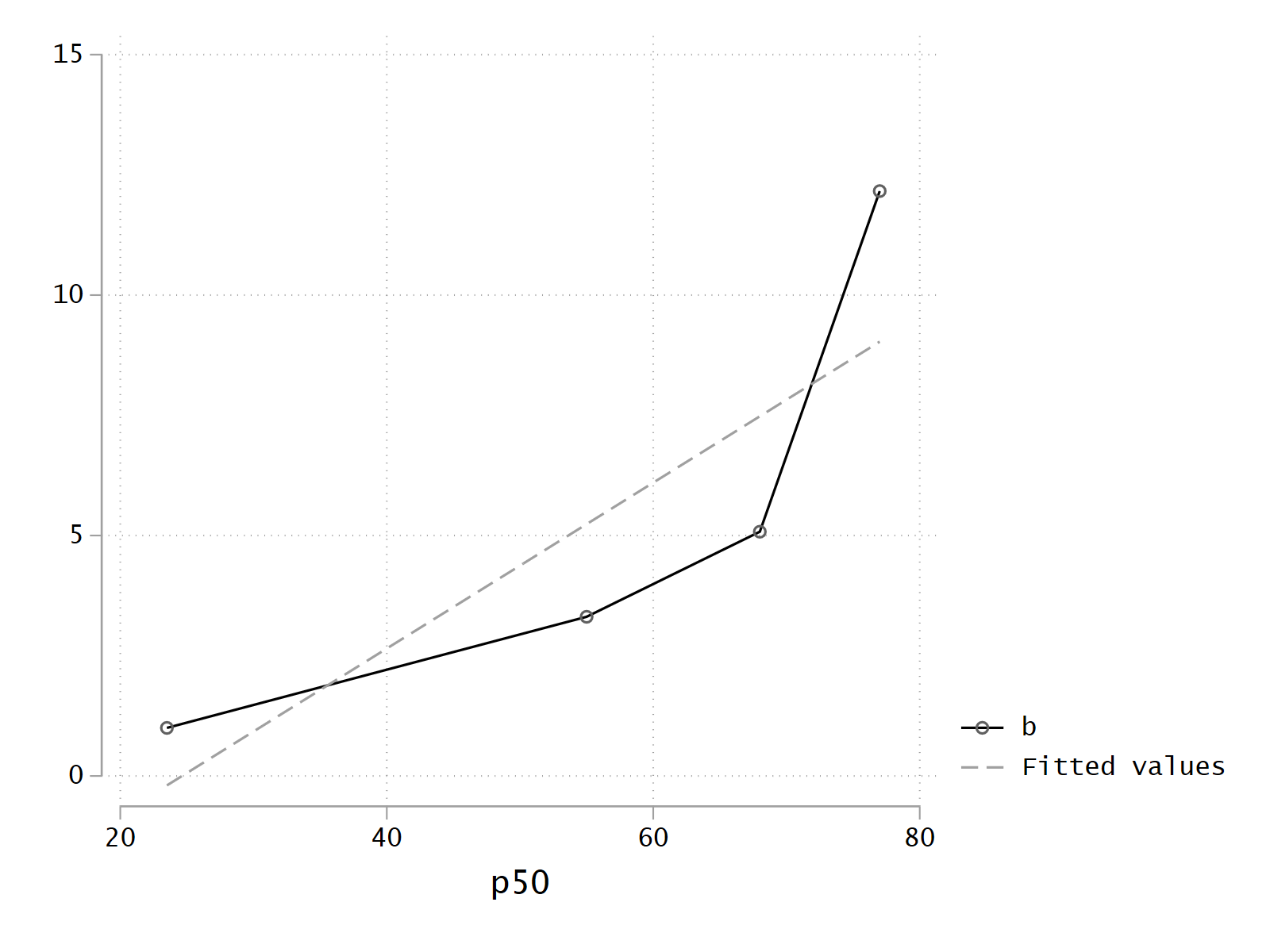
The (age, log odds) appear to be linear.
Smoothed Scatter Plot for age
This analysis are for univariable models only. So there are no adjustments possible.
The command -ksm- is replaced with the command -lowess-.
lowess sta age, logit name(age_smothed_scatter_plot, replace)

Also here monotonic/linear progression is present.
Conclusion for age
The effect of risk factor age is assumed linear.
The continuous risk factor sys
Quartile design for sys
The plot below indicates be non linearity.

However looking at odds ratios for the quartiles it might only being the last quartile that is signifcant.
Looking at estimates is seems fair to assume that only the fourth quarter is necessary in the model:
estout sys_grp, cells("b(fmt(2)) ci(fmt(2)) p(fmt(2))") varwidth(30) ///
        eform noabbrev keep(*sys*)
| sys_grp | |||||
|---|---|---|---|---|---|
| b | lower 95%ci | upper 95%ci | p | ||
| sta | 1bn.sys_grp | 1.00 | 1.00 | 1.00 | |
| 2.sys_grp | 0.92 | 0.28 | 3.00 | 0.90 | |
| 3.sys_grp | 1.02 | 0.32 | 3.24 | 0.98 | |
| 4.sys_grp | 0.19 | 0.04 | 0.89 | 0.04 |
This is confirmed below:
quietly logistic sta i.sys_grp age i.typ i.locd i.can i.pco i.ph
estimates store sys_grp_all
quietly logistic sta 4.sys_grp age i.typ i.locd i.can i.pco i.ph
estimates store sys_grp_4
estadd lrtest sys_grp_all
estout sys_grp_all sys_grp_4, cells("b(fmt(2)) ci(fmt(2)) p(fmt(2))") ///
        varwidth(30) noabbrev eform keep(*sys*) stats(lrtest_p, labels("LR p"))
| sys_grp_all | sys_grp_4 | ||||||||
|---|---|---|---|---|---|---|---|---|---|
| b | lower 95%ci | upper 95%ci | p | b | lower 95%ci | upper 95%ci | p | ||
| sta | 1bn.sys_grp | 1.00 | 1.00 | 1.00 | |||||
| 2.sys_grp | 0.92 | 0.28 | 3.00 | 0.90 | |||||
| 3.sys_grp | 1.02 | 0.32 | 3.24 | 0.98 | |||||
| 4.sys_grp | 0.19 | 0.04 | 0.89 | 0.04 | 0.19 | 0.04 | 0.81 | 0.02 | |
| LR p | 0.99 |
One can choose just to keep the fourth quartile in the model to handle the non linearity.
Smoothed Scatter Plot for sys

This appears not to be linear just like the Quartile design plot also indicated.
Quadratic effect for sys
Testing for quatradic effect can be done simply by adding the risk factor squared (c.sys#c.sys) to the model and do a likelihood ratio test for the squared term.
quietly logistic sta sys c.sys#c.sys age i.typ i.locd i.can i.pco i.ph
estimates store sys_quadratic
quietly logistic sta sys age i.typ i.locd i.can i.pco i.ph
estimates store sys_linear
estadd lrtest sys_quadratic
estout sys_quadratic sys_linear, cells("b(fmt(2)) ci(fmt(2)) p(fmt(2))") ///
        varwidth(30) noabbrev eform keep(*sys*)  stats(lrtest_p, labels("LR P value"))
| sys_quadratic | sys_linear | ||||||||
|---|---|---|---|---|---|---|---|---|---|
| b | lower 95%ci | upper 95%ci | p | b | lower 95%ci | upper 95%ci | p | ||
| sta | sys | 0.98 | 0.91 | 1.04 | 0.49 | 0.99 | 0.97 | 1.00 | 0.04 |
| c.sys#c.sys | 1.00 | 1.00 | 1.00 | 0.79 | |||||
| LR p | 0.79 |
There seems to be no quadratic effect.
Modelling non linearity with cubic splines
The dependency of sys might not be quadratic. More complex dependencies can be modelled by restricted cubic splines.
First cubic splines are generated by -mkspline-. Here the sys is modelled by 4 coherent cubic functions between the 5 knots. outside the first and last knot the sys is assumed to be linear.
mkspline sys_csp = sys, nknots(5) cubic
Then risk factor sys is replaced by the 4 variables generated by -mkspline-. However, the first variable is always the identity, so sys = sys_csp1.
Testing linearity is then at matter of testing the other generated variables equal to 0.
quietly logistic sta sys_csp* age i.typ i.locd i.can i.pco i.ph
estimates store sys_csp
quietly logistic sta sys_csp1 age i.typ i.locd i.can i.pco i.ph
estimates store sys_linear
estadd lrtest sys_csp
estout sys_csp sys_linear, cells("b(fmt(2)) ci(fmt(2)) p(fmt(2))") ///
        varwidth(30) noabbrev eform keep(sys*) stats(lrtest_p, labels("LR p"))
| sys_csp | sys_linear | ||||||||
|---|---|---|---|---|---|---|---|---|---|
| b | lower 95%ci | upper 95%ci | p | b | lower 95%ci | upper 95%ci | p | ||
| sta | sys_csp1 | 0.95 | 0.89 | 1.01 | 0.10 | 0.99 | 0.97 | 1.00 | 0.04 |
| sys_csp2 | 1.32 | 0.90 | 1.94 | 0.16 | |||||
| sys_csp3 | 0.24 | 0.03 | 2.00 | 0.19 | |||||
| sys_csp4 | 6.71 | 0.26 | 170.31 | 0.25 | |||||
| LR p | 0.54 |
The p-value from the likelihood ratio test is .
So there is no significant non linear effect according to this analysis.
Modelling non linearity with fractional polymials
In Stata there is a command for doing fractional polymials all in one step. The idea is to generate an optimal set of transformed variables of sys (default 2) in optimal powers.
The set of optimal variables replaces the original variable in a regression.
In the output there is a test of linearity
The p-value for the partial F test comparing the models and the lowest deviance model is given in the P(*) column.
fp <sys>, replace: logistic sta <sys> age i.typ i.locd i.can i.pco
(fitting 44 models)
(....10%....20%....30%....40%....50%....60%....70%....80%....90%....100%)

Fractional polynomial comparisons:
-------------------------------------------------------------------
             | Test              Deviance
         sys |   df   Deviance       diff.       P   Powers
-------------+-----------------------------------------------------
     omitted |    4    137.109      4.835    0.305
      linear |    3    132.881      0.608    0.895   1
       m = 1 |    2    132.784      0.510    0.775   .5
       m = 2 |    0    132.274      0.000       --   -2 -2
-------------------------------------------------------------------
Note: Test df is degrees of freedom, and P = P > chi2 is sig. level
      for tests comparing models vs. model with m = 2 based on
      deviance difference, chi2.

Logistic regression                                     Number of obs =    200
                                                        LR chi2(7)    =  67.89
                                                        Prob > chi2   = 0.0000
Log likelihood = -66.136762                             Pseudo R2     = 0.3392

--------------------------------------------------------------------------------------
                 sta | Odds ratio   Std. err.      z    P>|z|     [95% conf. interval]
---------------------+----------------------------------------------------------------
               sys_1 |      0.000      0.000    -1.62    0.10        0.000           .
               sys_2 |          .          .     1.72    0.08        0.000           .
                 age |      1.040      0.014     2.97    0.00        1.013       1.066
                     |
                 typ |
          emergency  |     21.049     20.049     3.20    0.00        3.254     136.149
                     |
                locd |
coma or deep stupor  |     56.550     56.272     4.06    0.00        8.043     397.601
                     |
                 can |
                yes  |     10.042      9.112     2.54    0.01        1.696      59.453
                     |
                 pco |
                >45  |      0.239      0.217    -1.58    0.11        0.040       1.415
               _cons |      0.000      0.000    -5.29    0.00        0.000       0.005
--------------------------------------------------------------------------------------
Note: _cons estimates baseline odds.
From P(*) in the Fractional polynomial comparisons it is seen that sys can ignored totally.
Conclusion for sys
There is no nonlinear effect of sys, but there seems to be an effect when is in the highest quarter.
Conclusion
After defining a variable for the upper quarter of systolic blood preasure:
generate sys_grp_4q = (sys_grp == 4) if !missing(sys_grp)
label variable sys_grp_4q "4th quarter systolic BP"
label define sys_grp_4q 0 "No" 1 "Yes"
the final model is chosen to be
quietly logistic sta sys_grp_4q age i.typ i.locd i.can i.pco i.ph
estimates store sys_grp_4
estout sys_grp_4, cells("b(fmt(2)) ci(fmt(2)) p(fmt(2))") varwidth(30) ///
        drop(0.*) eform noabbrev
| sys_grp_4 | |||||
|---|---|---|---|---|---|
| b | lower 95%ci | upper 95%ci | p | ||
| sta | sys_grp_4q | 0.19 | 0.04 | 0.81 | 0.02 |
| age | 1.05 | 1.02 | 1.08 | 0.00 | |
| 1.typ | 18.92 | 2.98 | 120.05 | 0.00 | |
| 1.locd | 113.93 | 13.48 | 963.14 | 0.00 | |
| 1.can | 10.45 | 1.93 | 56.50 | 0.01 | |
| 1.pco | 0.11 | 0.02 | 0.74 | 0.02 | |
| 1.ph | 6.44 | 1.16 | 35.85 | 0.03 | |
| _cons | 0.00 | 0.00 | 0.01 | 0.00 |
Examining the final fit of the model
Pearson or Hosmer-Lemeshow goodness-of-fit test
The postestimation command -estat gof- performs the Hosmer-Lemeshow goodness-of-fit test in Stata when the option group is set with a number. A depreciated command doing the same is -lfit-.
estat gof, table group(8)
note: obs collapsed on 8 quantiles of estimated probabilities.

Goodness-of-fit test after logistic model
Variable: sta

  Table collapsed on quantiles of estimated probabilities
  +--------------------------------------------------------+
  | Group |   Prob | Obs_1 | Exp_1 | Obs_0 | Exp_0 | Total |
  |-------+--------+-------+-------+-------+-------+-------|
  |     1 | 0.0103 |     0 |   0.1 |    25 |  24.9 |    25 |
  |     2 | 0.0316 |     0 |   0.5 |    25 |  24.5 |    25 |
  |     3 | 0.0438 |     2 |   0.9 |    23 |  24.1 |    25 |
  |     4 | 0.0916 |     2 |   1.6 |    23 |  23.4 |    25 |
  |     5 | 0.1773 |     4 |   3.3 |    21 |  21.7 |    25 |
  |-------+--------+-------+-------+-------+-------+-------|
  |     6 | 0.2886 |     4 |   5.9 |    22 |  20.1 |    26 |
  |     7 | 0.4547 |     9 |   8.6 |    15 |  15.4 |    24 |
  |     8 | 0.9832 |    19 |  19.0 |     6 |   6.0 |    25 |
  +--------------------------------------------------------+

 Number of observations =    200
       Number of groups =      8
Hosmer–Lemeshow chi2(6) =   3.01
            Prob > chi2 = 0.8075
It is worth noting that the first 5 expected values in the event of death at discharge from hospital all are below 5. Usually in chisquare test the expected values are required to be above 5.
It the option group is not set -estat gof- does the Pearson test.
estat gof
Goodness-of-fit test after logistic model
Variable: sta

      Number of observations =    200
Number of covariate patterns =    145
           Pearson chi2(137) =  81.72
                 Prob > chi2 = 1.0000
The Hosmer-Lemeshow goodness-of-fit test is critised being dependent on the number of groups chosen for the test.
Eg Long & Freese shows on page 223 an example of opposite conclusions depending on whether the numbers of groups are 9 or 11 (model does not fit, p ~ 3%) in contrast to if the number is 10 (model fits, p ~ 8%). In number of groups from 5 to 15 5 groups returns a p value of 25.7% whereas 12 groups returns a p value of 0.7%. So there is quite a variation depending of group number.
However in this dataset the variation does not lead to different conclusions with respect to fit.
| df | chi2 | p | ||
|---|---|---|---|---|
| Number | 10 | 8 | 2 | 0.98 |
| of | 15 | 13 | 9 | 0.77 |
| groups | 20 | 18 | 12 | 0.85 |
| 25 | 23 | 18 | 0.77 | |
| 30 | 28 | 17 | 0.95 | |
| 35 | 33 | 20 | 0.96 | |
| 40 | 38 | 22 | 0.98 |
Other measures of fit
In Long & Freese a command -fitstat- is demonstrated.
It needs to be installed by findit spost9 or findit spost13 depending on
your Stata version.
As guidelines all R squared has the same interpretation being between 0 and 1 and measures the variation explained by the model.
The Akaike information criterion (AIC) and the Bayesian information criterion (BIC) are both goodness of fit measures penalising the number of parameters used in the model to use for comparison of different models (the lowest value being best).
fitstat
                         |    logistic
-------------------------+-------------
Log-likelihood           |
                   Model |     -63.233
          Intercept-only |    -100.080
-------------------------+-------------
Chi-square               |
        Deviance(df=192) |     126.466
                LR(df=7) |      73.695
                 p-value |       0.000
-------------------------+-------------
R2                       |
                McFadden |       0.368
      McFadden(adjusted) |       0.288
            Cox-Snell/ML |       0.308
  Cragg-Uhler/Nagelkerke |       0.487
                   Efron |       0.388
                Tjur's D |       0.389
                   Count |       0.875
         Count(adjusted) |       0.375
-------------------------+-------------
IC                       |
                     AIC |     142.466
        AIC divided by N |       0.712
               BIC(df=8) |     168.853
Residual plots
The recipe below is inspired by Dupont.
First restore the estimates for the selected model
estimates restore sys_grp_4
- Numbering the covariate patterns
predict J, number
label variable J "jth covariate pattern"
- Estimate the pi's for the covariate patterns
predict p, p
label variable p "Estimate of pi for the jth covariate pattern"
- Calculate Pearson (standardized) residuals
predict rstandard, rstandard
label variable rstandard "Pearson residuals"
- Calculate the Delta chi-squared influence statistic $$\Delta\chi_j^2 = \frac{Pearson \, residual_j^2}{1-leverage_j}$$
predict dx2, dx2
label variable dx2 "Delta chi-squared influence"
- Calculate the Delta-beta influence
predict dbeta, dbeta
label variable dbeta "Delta-Beta influence"
- For graph purposes separate the Delta chisquared depending on the sign of the Pearson residual
generate dx2_pos = dx2 if rstandard >= 0
generate dx2_neg = dx2 if rstandard < 0
- Do the graph
twoway ///
        (scatter dx2_pos p [weight=dbeta], symbol(oh) mlwidth(thick) color(black)) ///
        (scatter dx2_neg p [weight=dbeta], symbol(oh) mlwidth(thick) color(gs8)) ///
        (scatter dx2_pos p [weight=dbeta] if dx2_pos > 3, color(black) mlabel(J) mlabposition(3) msymbol(none) mlabgap(medium) mcolor(black)) ///
        (scatter dx2_neg p [weight=dbeta] if dx2_neg > 3, color(gs8) mlabel(J) mlabposition(3) msymbol(none) mlabgap(medium) mcolor(black)) ///
        , yline(3.84) legend(order(1 "Positive" 2 "Negative")) ///
        ytitle(Squared Std Pearson Residuals) ///
        name(sqr_std_P_res, replace)
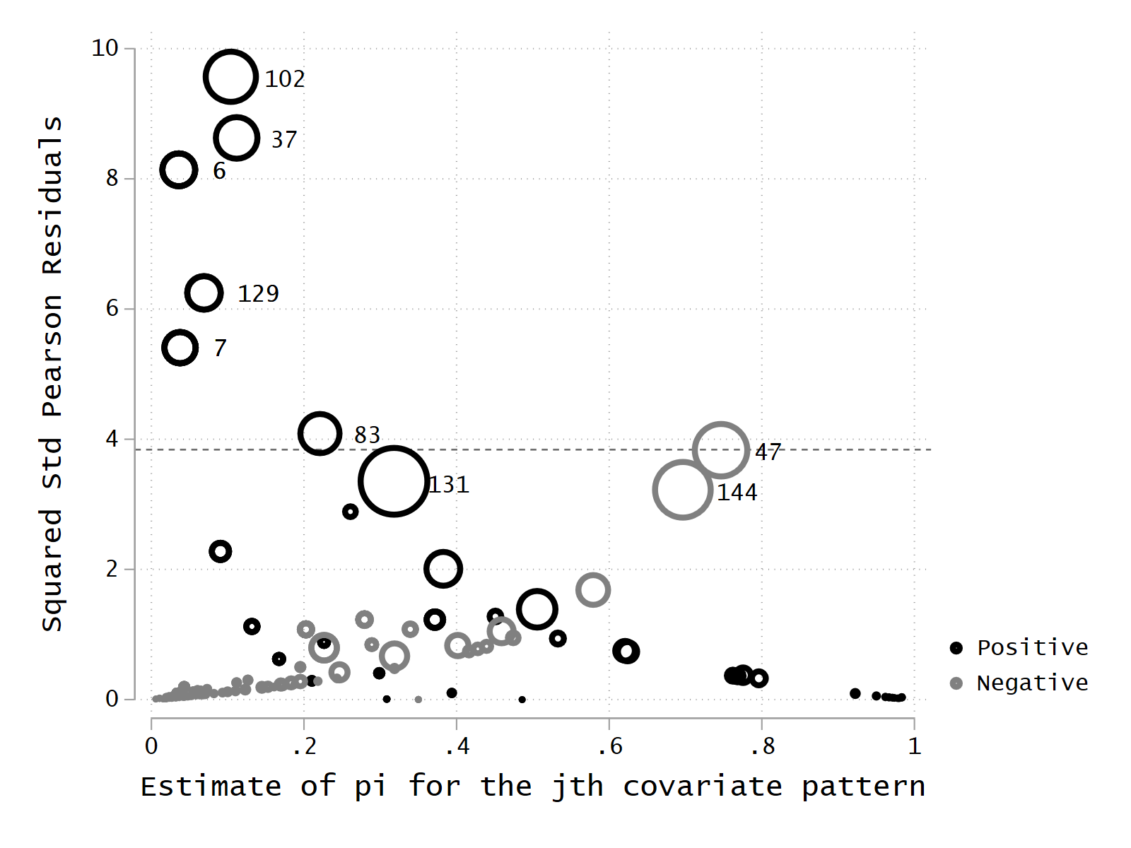
One could consider whether one or more of the influential covariate patterns should be ignored from the list below.
Or maybe it is possible to identify covariate patterns that the model predicts poorly.
sort dx2
keep sta sys_grp_4q age typ locd can pco ph dbeta dx2 p
list  if dx2 > 3.84
     +---------------------------------------------------------------------------------------------------------------------------------------------+
     |                         sta   age   can         typ       ph    pco                     locd   sys_g~4q           p         dx2       dbeta |
     |---------------------------------------------------------------------------------------------------------------------------------------------|
189. |  Dead at hospital discharge    75   yes    elective    >7.25   <=45   no coma or deep stupor          0   .22070255    4.052487   .59852388 |
190. | Alive at hospital discharge    20    no   emergency    >7.25   <=45   no coma or deep stupor          0   .03738583   5.3798264   .38055762 |
191. | Alive at hospital discharge    20    no   emergency    >7.25   <=45   no coma or deep stupor          0   .03738583   5.3798264   .38055762 |
192. |  Dead at hospital discharge    20    no   emergency    >7.25   <=45   no coma or deep stupor          0   .03738583   5.3798264   .38055762 |
193. | Alive at hospital discharge    20    no   emergency    >7.25   <=45   no coma or deep stupor          0   .03738583   5.3798264   .38055762 |
     |---------------------------------------------------------------------------------------------------------------------------------------------|
194. | Alive at hospital discharge    69    no   emergency    >7.25   <=45   no coma or deep stupor          1   .06873963   6.2190947   .43706282 |
195. |  Dead at hospital discharge    69    no   emergency    >7.25   <=45   no coma or deep stupor          1   .06873963   6.2190947   .43706282 |
196. |  Dead at hospital discharge    19    no   emergency    >7.25   <=45   no coma or deep stupor          0   .03573318   8.1105434    .4200881 |
197. | Alive at hospital discharge    19    no   emergency    >7.25   <=45   no coma or deep stupor          0   .03573318   8.1105434    .4200881 |
198. | Alive at hospital discharge    19    no   emergency    >7.25   <=45   no coma or deep stupor          0   .03573318   8.1105434    .4200881 |
     |---------------------------------------------------------------------------------------------------------------------------------------------|
199. |  Dead at hospital discharge    53    no   emergency   =<7.25    >45   no coma or deep stupor          0   .11155914   8.5918097   .67746894 |
200. |  Dead at hospital discharge    91    no   emergency    >7.25    >45   no coma or deep stupor          0   .10389305    9.523432   .99167298 |
     +---------------------------------------------------------------------------------------------------------------------------------------------+
Sensitivity and specificity
The command -estat classification- reports summary statistics like the classification table for the model. Note that the default cut-off in -estat classification- is "P(D) >= 0.5". It is possible to choose other cut-offs by the option cutoff.
A depreciated command doing the same is -lstat-.
estat classification
Logistic model for sta

              -------- True --------
Classified |         D            ~D  |      Total
-----------+--------------------------+-----------
     +     |        18             3  |         21
     -     |        22           157  |        179
-----------+--------------------------+-----------
   Total   |        40           160  |        200

Classified + if predicted Pr(D) >= .5
True D defined as sta != 0
--------------------------------------------------
Sensitivity                     Pr( +| D)   45.00%
Specificity                     Pr( -|~D)   98.13%
Positive predictive value       Pr( D| +)   85.71%
Negative predictive value       Pr(~D| -)   87.71%
--------------------------------------------------
False + rate for true ~D        Pr( +|~D)    1.88%
False - rate for true D         Pr( -| D)   55.00%
False + rate for classified +   Pr(~D| +)   14.29%
False - rate for classified -   Pr( D| -)   12.29%
--------------------------------------------------
Correctly classified                        87.50%
--------------------------------------------------
Last update: 2022-04-22, Stata version 17