Understanding mlogit and margins
Aim
The objective is to understand what multinomial regression -mlogit- returns. And to show how to report these results using the commands -margins-, -coefplot-, -mchange-, and -mchangeplot-. The last two commands are from the package spost13.
Other sources on -mlogit- in Stata:
Stata example dataset
"We have data on the type of health insurance available to 616 psychologically depressed subjects in the United States (Tarlov et al. 1989; Wells et al. 1989). The insurance is categorized as either an indemnity plan (that is, regular fee-for-service insurance, which may have a deductible or coinsurance rate) or a prepaid plan (a fixed up-front payment allowing subsequent unlimited use as provided, for instance, by an HMO). The third possibility is that the subject has no insurance whatsoever. We wish to explore the demographic factors associated with each subject’s insurance choice.
One of the demographic factors in our data is the race of the participant, coded as white or nonwhite.
Retrieving the dataset and variables.
use patid age male nonwhite insure site using http://www.stata-press.com/data/r15/sysdsn1.dta, clear
| Name | Index | Label | Value Label Name | Format | Value Label Values | n | unique | missing |
|---|---|---|---|---|---|---|---|---|
| patid | 1 | %9.0g | 644 | 644 | 0 | |||
| age | 2 | NEMC (ISCNRD-IBIRTHD)/365.25 | %10.0g | 643 | 632 | 1 | ||
| male | 3 | NEMC PATIENT MALE | %8.0g | 644 | 2 | 0 | ||
| nonwhite | 4 | %9.0g | 644 | 2 | 0 | |||
| insure | 5 | insure | %9.0g | 1 "Indemnity" 2 "Prepaid" 3 "Uninsure" | 616 | 3 | 28 | |
| site | 6 | %9.0g | 644 | 3 | 0 |
Labelling data.
label variable nonwhite "Race"
label define nonwhite 0 "White" 1 "Non white"
label values nonwhite nonwhite
What are the estimates from -mlogit-
The estimates from are odds ratios (or log odds ratios) comparing the odds (or log odds) of current value of the outcome with the reference value of the outcome dependent on the exposure variable.
First the -mlogit- command itself.
Both crude and adjusted (male and age) estimates of the effect of nonwhite on insure is estimated. With option rrr odds ratios are reported.
The estimates and their confidence intervals are gathered in a matrix tbl.
regmat, outcome(insure) exposure(i.nonwhite) adjustments("" "i.male c.age") ///
        drop(se p) decimals(4) label: mlogit, nolog baseoutcome(2) rrr
matrix tbl = r(regmat)
matrix roweq tbl = Prepaid Uninsure
For comparison more variables is needed.
First in order to compare the insure value Indemnity (1) with the reference (2) value Prepaid a new variable insure12.
Recoding is necessary since logit requires outcome variable to be zero/one. Note that the third value not used for comparison is set to missing.
generate insure12 = (insure == 1) if insure != 3 & !missing(insure)
label variable insure12 "Prepaid"
label define insure12 0 "Prepaid" 1 "Indemnity"
label values insure12 insure12
Then a logistic regression is done to get odds ratio estimates and their confidence intervals.
Estimates and confidence intervals are added to the matrix tbl.
regmat, outcome(insure12) exposure(i.nonwhite) adjustments("" "i.male c.age") ///
        drop(se p) decimals(4) label: logit, nolog or
matrix tbl = tbl \ r(regmat)
Now comparing the outcome value Uninsure (3) with the reference value Prepaid (2) is similar to the above.
generate insure32 = (insure == 3) if insure != 1 & !missing(insure)
label variable insure32 "Uninsure"
label define insure32 0 "Prepaid" 1 "Uninsure"
label values insure32 insure32
regmat, outcome(insure32) exposure(i.nonwhite) adjustments("" "i.male c.age") ///
        drop(se p) decimals(4) label: logit, nolog or
matrix tbl = tbl \ r(regmat)
Finally, below is the matrix tbl presented with the aggregated results from the different regressions.
| Adjustment 1 | Adjustment 2 | ||||||
|---|---|---|---|---|---|---|---|
| b | Lower 95% CI | Upper 95% CI | b | Lower 95% CI | Upper 95% CI | ||
| Prepaid | Race (Non white) | -0.6608 | -1.0836 | -0.2380 | -0.7313 | -1.1605 | -0.3021 |
| Uninsure | Race (Non white) | -0.2829 | -1.0624 | 0.4967 | -0.2980 | -1.0827 | 0.4868 |
| Prepaid | Race (Non white) | -0.6608 | -1.0836 | -0.2380 | -0.7158 | -1.1443 | -0.2873 |
| Uninsure | Race (Non white) | -0.2829 | -1.0624 | 0.4967 | -0.2923 | -1.0764 | 0.4919 |
Visualising estimates from -mlogit-
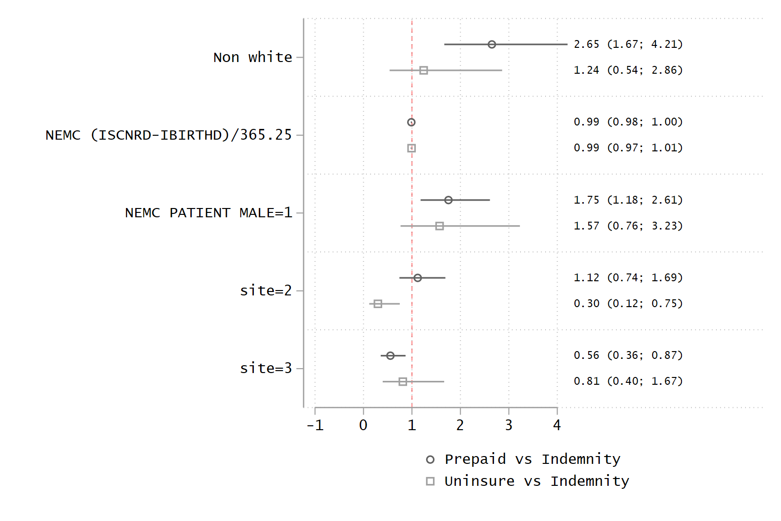
Let's look at the estimate of the effects of nonwhite on insure adjusted for age, gender and site.
mlogit insure b0.nonwhite c.age i.male i.site, rrr base(1) nolog
estimates store mlogit_1
The command -coefplot- is an excellent tool to visualise estimates and their confidence interval.
coefplot ///
        (,keep(*Pr*:*) drop(_cons) label(Prepaid vs Indemnity)) ///
        (,keep(*Un*:*) drop(_cons) label(Uninsure vs Indemnity)) ///
        , eform xline(1, lcolor(red%40)) legend(rows(2) ring(1) position(6)) generate ///
        name(coefplot1, replace)
Generated variables:
Variable      Storage   Display    Value
    name         type    format    label      Variable label
---------------------------------------------------------------------------------------------------------------------------------------------------------------------------------------------------------------------------------------------------------------
__by            byte    %10.0g     __by       subgraph ID
__plot          byte    %10.0g     __plot     plot ID
__at            float   %10.0g                plot position (category axis)
__mlbl          str1    %9s                   marker label
__mlpos         byte    %10.0g                marker label position
__b             double  %10.0g                coefficient
__V             double  %10.0g                variance
__se            double  %10.0g                standard error
__t             double  %10.0g                t or z statistic
__df            byte    %10.0g                degrees of freedom
__pval          double  %10.0g                p-value
__ll1           double  %10.0g                CI1: lower limit
__ul1           double  %10.0g                CI1: upper limit
As seen in the returned text in the log the option generate saves a set of variables with prefix __. Some of these are used to generate a variable label.
replace __mlbl = string(__b, "%6.2f") + " (" + string(__ll1, "%6.2f") + "; " ///
        + string(__ul1, "%6.2f") + ")" if !missing(__b)
The estimates and their confidence intervals are to be placed nicely above one another to the right in the graph. The x-value are to be the rounded maximum upper confidence interval limit (__ull).
summarize __ul1
replace __mlpos = round(r(max), 0.1) if !missing(__b)
addplot: scatter __at __mlpos, ms(i) mlabel(__mlbl) mlabsize(vsmall) ///
        xlabel(-1(1)4) xscale(range(-1 8)) yticks(0.5(1)5.5) ///
        legend(order(2 `"Prepaid vs Indemnity"' 4 `"Uninsure vs Indemnity"'))
Margins and mlogit
Understanding margins is easiest when there is only one main effect in the regression.
mlogit insure b0.nonwhite, rrr base(1) nolog
Multinomial logistic regression                         Number of obs =    616
                                                        LR chi2(2)    =   9.62
                                                        Prob > chi2   = 0.0081
Log likelihood = -551.78348                             Pseudo R2     = 0.0086

------------------------------------------------------------------------------
      insure |        RRR   Std. err.      z    P>|z|     [95% conf. interval]
-------------+----------------------------------------------------------------
Indemnity    |  (base outcome)
-------------+----------------------------------------------------------------
Prepaid      |
    nonwhite |
  Non white  |      1.936      0.418     3.06    0.00        1.269       2.955
       _cons |      0.829      0.078    -2.00    0.05        0.690       0.996
-------------+----------------------------------------------------------------
Uninsure     |
    nonwhite |
  Non white  |      1.459      0.595     0.93    0.35        0.656       3.244
       _cons |      0.143      0.026   -10.90    0.00        0.101       0.203
------------------------------------------------------------------------------
Note: _cons estimates baseline relative risk for each outcome.
estimates store mlogit_main
The LR test in -mlogit- the same as a classical LR chisquare test for independence. Compare to the -tabulate- output below.
Then -margins- predicts the probabilities of the outcome (insure) given the exposure (nonwhite), ie the expected probability $$P(insure|nonwhite)$$.
margins nonwhite, cformat(%6.4f)
Adjusted predictions                                       Number of obs = 616
Model VCE: OIM

1._predict: Pr(insure==Indemnity), predict(pr outcome(1))
2._predict: Pr(insure==Prepaid), predict(pr outcome(2))
3._predict: Pr(insure==Uninsure), predict(pr outcome(3))

-----------------------------------------------------------------------------------
                  |            Delta-method
                  |     Margin   std. err.      z    P>|z|     [95% conf. interval]
------------------+----------------------------------------------------------------
_predict#nonwhite |
         1#White  |     0.5071     0.0225    22.57    0.00       0.4630      0.5511
     1#Non white  |     0.3554     0.0435     8.17    0.00       0.2701      0.4407
         2#White  |     0.4202     0.0222    18.94    0.00       0.3767      0.4637
     2#Non white  |     0.5702     0.0450    12.67    0.00       0.4820      0.6585
         3#White  |     0.0727     0.0117     6.23    0.00       0.0499      0.0956
     3#Non white  |     0.0744     0.0239     3.12    0.00       0.0276      0.1211
-----------------------------------------------------------------------------------
compared to the column percentages from e.g. -tabulate-.
tabulate insure nonwhite, col lrchi2
+-------------------+
| Key               |
|-------------------|
|     frequency     |
| column percentage |
+-------------------+

           |         Race
    insure |     White  Non white |     Total
-----------+----------------------+----------
 Indemnity |       251         43 |       294
           |     50.71      35.54 |     47.73
-----------+----------------------+----------
   Prepaid |       208         69 |       277
           |     42.02      57.02 |     44.97
-----------+----------------------+----------
  Uninsure |        36          9 |        45
           |      7.27       7.44 |      7.31
-----------+----------------------+----------
     Total |       495        121 |       616
           |    100.00     100.00 |    100.00

 Likelihood-ratio chi2(2) =   9.6231   Pr = 0.008
The marginal effect (risk difference): $$P(insure|nonwhite = Non white) - P(insure|nonwhite = White)$$ can found by
margins r.nonwhite, cformat(%6.4f)
Contrasts of adjusted predictions                          Number of obs = 616
Model VCE: OIM

1._predict: Pr(insure==Indemnity), predict(pr outcome(1))
2._predict: Pr(insure==Prepaid), predict(pr outcome(2))
3._predict: Pr(insure==Uninsure), predict(pr outcome(3))

-----------------------------------------------------------
                        |         df        chi2     P>chi2
------------------------+----------------------------------
      nonwhite@_predict |
(Non white vs White) 1  |          1        9.60     0.0020
(Non white vs White) 2  |          1        8.94     0.0028
(Non white vs White) 3  |          1        0.00     0.9504
                 Joint  |          2       10.02     0.0067
-----------------------------------------------------------

-------------------------------------------------------------------------
                        |            Delta-method
                        |   Contrast   std. err.     [95% conf. interval]
------------------------+------------------------------------------------
      nonwhite@_predict |
(Non white vs White) 1  |    -0.1517     0.0490       -0.2477     -0.0557
(Non white vs White) 2  |     0.1500     0.0502        0.0517      0.2484
(Non white vs White) 3  |     0.0017     0.0266       -0.0504      0.0537
-------------------------------------------------------------------------
Or by:
margins, dydx(nonwhite) post
Conditional marginal effects                               Number of obs = 616
Model VCE: OIM

dy/dx wrt: 1.nonwhite

1._predict: Pr(insure==Indemnity), predict(pr outcome(1))
2._predict: Pr(insure==Prepaid), predict(pr outcome(2))
3._predict: Pr(insure==Uninsure), predict(pr outcome(3))

------------------------------------------------------------------------------
             |            Delta-method
             |      dy/dx   std. err.      z    P>|z|     [95% conf. interval]
-------------+----------------------------------------------------------------
0.nonwhite   |  (base outcome)
-------------+----------------------------------------------------------------
1.nonwhite   |
    _predict |
          1  |     -0.152      0.049    -3.10    0.00       -0.248      -0.056
          2  |      0.150      0.050     2.99    0.00        0.052       0.248
          3  |      0.002      0.027     0.06    0.95       -0.050       0.054
------------------------------------------------------------------------------
Note: dy/dx for factor levels is the discrete change from the base level.
Since the marginal effects are the risk differences between two sets of column probabilities where each set sums to one, we have that marginal effects (risk differences) per construction sums to zero.
Option post is needed for the coming -coefplot- command.
A coefplot can be made by:
coefplot (, keep(*:1._predict) label(Indemnity)) ///
         (, keep(*:2._predict) label(Prepaid))   ///
         (, keep(*:3._predict) label(Uninsure))  ///
    , swapnames xline(0) legend(cols(1)) ///
        mlabel(string(@b, "%5.2f") + " (" + string(@ll, "%5.2f") + "; " + string(@ul, "%5.2f") + ")") ///
        mlabposition(12) mlabsize(vsmall) name(coefplot2, replace)

Similar results can be achieved by the spost13 commands -mchange-.
estimates restore mlogit_main
mchange, stats(ci)
mlogit: Changes in Pr(y) | Number of obs = 616

Expression: Pr(insure), predict(outcome())

                    | Indemnity    Prepaid   Uninsure
--------------------+---------------------------------
nonwhite            |
 Non white vs White |    -0.152      0.150      0.002
                 LL |    -0.248      0.052     -0.050
                 UL |    -0.056      0.248      0.054

Average predictions

             | Indemnity    Prepaid   Uninsure
-------------+---------------------------------
  Pr(y|base) |     0.477      0.450      0.073
Last update: 2022-04-22, Stata version 17